Building LCS models with OpenMx
In OpenMx, it is possible to specify a Structural Equation Model either by writing the entire matrices (with mxMatrix()), or by writing only the paths (with mxPath()). We will use the latter because it is faster to specify with longitudinal data, and usually more intuitive for researchers. First, install the package if necessary:
install.packages("OpenMx")To build a model in OpenMx, we use the function mxModel() with the following arguments:
model: Usemodel = "LCS_model"to create a new model with named “LCS_model”.type: Usetype = RAM(Reticular Action Model), to define the model in terms of single-headed and double-headed paths between variables, just as in a path diagram.manifestVars = c("Y1", "Y2", "Y3"...): Include the names of the observed variables in your database.latentVars = c("y1", "y2", "y3"...): Include the names that you will use to identify the latent variables in the model.mxData(observed = dfwide, type="raw"): Select your database and indicate that it contains observed scores by setting the argument type toraw(it is also possible to use covariance or correlation matrices as inputs).
Once we have finished the preparations, building the model is very intuitive. All paths are defined through the function mxPath(). The arguments from and to are used to indicate the origins and endings of the paths, arrows to indicate regression (=1) or covariance (=2), free to fix (=FALSE) or freely estimate (=TRUE) the parameters defining the paths, values to indicate the value of a fixed parameter (when free=FALSE) or to set to set an initial value for a free parameter (when free=TRUE), and labels to name the parameter defining the paths. Using the same label for multiple paths implies imposing an equality constraint, meaning that a single parameter will be estimated across those paths.
An important advantage of OpenMx is that it does not require to define each single path separately. For example, it is possible to define all the paths from y(t - 1) to y(t) just by specifying from=latent_y[1:(t-1)], to=latent_y[2:t] inside mxPath(), where latent_y is a string that contains the names of the latent states of y across all time points.
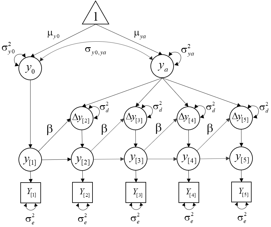
The Univariate LCS model
Single indicator
Obtain the example database here: Download LCSdata.txt
We will estimate the following model:
Step 1. Load the package and database:
library(OpenMx)
dfwide <- read.table("LCSdata.txt")
Step 2. Define the variables of the model:
Tmax <- 5 # Number of measurement occasions
colnames(dfwide) <- paste0("Y", 1:Tmax)
# Initial factor:
y0 <- "y0"
# Additive component:
ya <- "ya"
# Manifest scores:
manif_Y <- paste0("Y", 1:Tmax)
# Latent scores:
latent_y <- paste0("y", 1:Tmax)
# Latent changes:
change_y <- paste0("Delta_", 2:Tmax)
Step 3. Build the model:
LCS.model <- mxModel("Univariate LCS", type = "RAM",
               manifestVars = manif_Y,
               latentVars = c(y0, ya, latent_y, change_y),
               mxData(observed = dfwide, type="raw"),

    ### LATENT STRUCTURE
      # 1 -> Initial factor and additive component (means)
      # “one” is used to define intercepts. In this case, the paths from “one” to y0 and ya represent the means of these latent variables.
               mxPath(from="one", to=c(y0, ya),
                      arrows=1, free=TRUE, values= 0, labels=c("meany0", "meanya")),

               # (Co)variances of the initial factor and additive component
               mxPath(from=y0, arrows=2, free=TRUE, values=0, labels="vary0"),
               mxPath(from=ya, arrows=2, free=TRUE, values=0, labels="varya"),
               mxPath(from=y0, to=ya,
                      arrows=2, free=TRUE, values=0, labels="covy0ya"),

               # Initial factor -> Initial latent score
               mxPath(from=y0, to=latent_y[1], arrows=1, free=FALSE, values=1),

               # Latent[t-1] -> Latent[t]
               mxPath(from=latent_y[1:(Tmax-1)], to=latent_y[2:Tmax],
                      arrows=1, free=FALSE, values=1),

               # Additive component -> Change[t] (alpha = 1)
               mxPath(from=ya, to=change_y, arrows=1, free=FALSE, values=1),

               # Latent[t-1] -> Change[t] (self-feedback)
               mxPath(from=latent_y[1:(Tmax-1)], to=change_y,
                      arrows=1, free=TRUE, values=0, labels="beta"),

               # Change -> Latent
               mxPath(from=change_y, to=latent_y[2:Tmax], arrows=1, free=FALSE, values=1),

    ### MEASUREMENT STRUCTURE
               # Latent -> Manifest
               mxPath(from=latent_y, to=manif_Y, arrows=1, free=FALSE, values=1),

               # Measurement error variance
               mxPath(from=manif_Y, arrows=2, free=TRUE, values=.5, labels="merY"))
Step 4. Estimate the model parameters:
LCS.fit <- mxRun(LCS.model)Click here to see the results
summary(LCS.fit)## Summary of Univariate LCS
##
## free parameters:
## name matrix row col Estimate Std.Error A
## 1 beta A Delta_2 y1 -0.23438720 0.010998162
## 2 merY S Y1 Y1 0.32064158 0.005884500
## 3 vary0 S y0 y0 0.64509081 0.028010421
## 4 covy0ya S y0 ya 0.11723448 0.009873330
## 5 varya S ya ya 0.09966682 0.006198747
## 6 meany0 M 1 y0 -1.15984663 0.021784269
## 7 meanya M 1 ya -0.94513129 0.023805748
##
## Model Statistics:
## | Parameters | Degrees of Freedom | Fit (-2lnL units)
## Model: 7 9893 23280.07
## Saturated: 20 9880 NA
## Independence: 10 9890 NA
## Number of observations/statistics: 1980/9900
##
## Information Criteria:
## | df Penalty | Parameters Penalty | Sample-Size Adjusted
## AIC: 3494.069 23294.07 23294.13
## BIC: -51816.231 23333.20 23310.97
## To get additional fit indices, see help(mxRefModels)
## timestamp: 2021-04-18 20:26:58
## Wall clock time: 0.1585219 secs
## optimizer: SLSQP
## OpenMx version number: 2.19.1
## Need help? See help(mxSummary)Stochastic LCS model
It is possible to extend the previous model to include innovation variance by just adding a new mxPath() to the already built LCS.model:
stoch_LCS.model <- mxModel(LCS.model, # call the previous model
                           # Dynamic error variance
                           mxPath(from=change_y, arrows=2, free=TRUE, values=0, labels="derY"))

# Run the new model:
stoch_LCS.fit <- mxRun(stoch_LCS.model)
Click here to see the results
summary(stoch_LCS.fit)## Summary of Univariate LCS
##
## free parameters:
## name matrix row col Estimate Std.Error A
## 1 beta A Delta_2 y1 -0.23978246 0.011700562
## 2 merY S Y1 Y1 0.26099004 0.011663449
## 3 vary0 S y0 y0 0.66218447 0.028157304
## 4 covy0ya S y0 ya 0.11338030 0.010260152
## 5 varya S ya ya 0.08076624 0.007491957
## 6 derY S Delta_2 Delta_2 0.10208647 0.018716374
## 7 meany0 M 1 y0 -1.15671290 0.021407325
## 8 meanya M 1 ya -0.95608397 0.025150281
##
## Model Statistics:
## | Parameters | Degrees of Freedom | Fit (-2lnL units)
## Model: 8 9892 23247.73
## Saturated: 20 9880 NA
## Independence: 10 9890 NA
## Number of observations/statistics: 1980/9900
##
## Information Criteria:
## | df Penalty | Parameters Penalty | Sample-Size Adjusted
## AIC: 3463.733 23263.73 23263.81
## BIC: -51840.976 23308.46 23283.04
## To get additional fit indices, see help(mxRefModels)
## timestamp: 2021-04-18 20:26:58
## Wall clock time: 0.1607468 secs
## optimizer: SLSQP
## OpenMx version number: 2.19.1
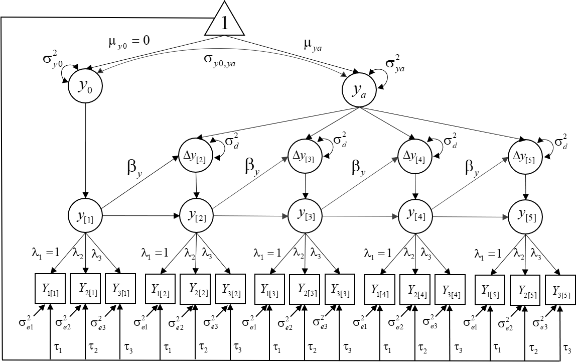
## Need help? See help(mxSummary)Multiple indicators
Obtain the example database here: Download MILCSdata.txt
We will estimate the following model:
Step 1. Load the package and database:
library(OpenMx)
dfwide <- read.table("MILCSdata.txt")
Step 2. Define the variables of the model:
Tmax <- 5 # Number of measurement occasions
# Create the labels for the latent state at t=0, the additive component, each one of the observed indicators, the latent scores, and the latent changes:
y0 <- "y0"
ya <- "ya"
indic_Y1 <- paste0("Y1_t", 1:Tmax)
indic_Y2 <- paste0("Y2_t", 1:Tmax)
indic_Y3 <- paste0("Y3_t", 1:Tmax)
latent_y <- paste0("y", 1:Tmax)
change_y <- paste0("Delta_", 2:Tmax)
Step 3. Build the model:
MI_LCS.model <- mxModel("Multiple Indicator LCS", type = "RAM",
         manifestVars = c(indic_Y1, indic_Y2, indic_Y3),
         latentVars = c(y0, ya, latent_y, change_y),
         mxData(observed = dfwide, type="raw"),

   ### LATENT STRUCTURE
         # 1 -> Initial factors and additive components (means)
         # Note that we only estimate the latent mean of the additive component
         mxPath(from="one", to=ya, arrows=1, free=TRUE, values= 0, labels="meanya"),

         # (Co)variances of the initial factors and additive components (covariance structure)
         mxPath(from=y0, arrows=2, free=TRUE, values=0, labels="vary0"),
         mxPath(from=ya, arrows=2, free=TRUE, values=0, labels="varya"),
         mxPath(from=y0, to=ya,
                arrows=2, free=TRUE, values=0, labels="covy0ya"),

         # Initial factor -> Initial latent score
         mxPath(from=y0, to=latent_y[1], arrows=1, free=FALSE, values=1),

         # Latent[t-1] -> Latent[t]
         mxPath(from=latent_y[1:(Tmax-1)], to=latent_y[2:Tmax],
                arrows=1, free=FALSE, values=1),

         # Additive component -> Change (alpha = 1)
         mxPath(from=ya, to=change_y, arrows=1, free=FALSE, values=1),

         # Latent[t-1] -> Change[t] (self-feedback)
         mxPath(from=latent_y[1:(Tmax-1)], to=change_y,
                arrows=1, free=TRUE, values=0, labels="beta"),

         # Change -> Latent
         mxPath(from=change_y, to=latent_y[2:Tmax], arrows=1, free=FALSE, values=1),

         ## For the stochastic version, include:
         # Dynamic error variance (time-invariant)
         mxPath(from=change_y, arrows=2, free=TRUE, values=0, labels="derY"),

   ### MEASUREMENT STRUCTURE
         # Factor loadings: Configural and weak invariance
         mxPath(from=latent_y, to=indic_Y1, arrows=1, free=FALSE, values=1, labels="lambda_Y1"),
         mxPath(from=latent_y, to=indic_Y2, arrows=1, free=TRUE, values=0, labels="lambda_Y2"),
         mxPath(from=latent_y, to=indic_Y3, arrows=1, free=TRUE, values=0, labels="lambda_Y3"),

         # Intercepts of the indicators: Strong invariance
         mxPath(from="one", to=indic_Y1, arrows=1, free=TRUE, values=0, labels="tau_Y1"),
         mxPath(from="one", to=indic_Y2, arrows=1, free=TRUE, values=0, labels="tau_Y2"),
         mxPath(from="one", to=indic_Y3, arrows=1, free=TRUE, values=0, labels="tau_Y3"),

         # Measurement error variances (time-invariant)
         mxPath(from=indic_Y1, arrows=2, free=TRUE, values=0, labels="mer_Y1"),
         mxPath(from=indic_Y2, arrows=2, free=TRUE, values=0, labels="mer_Y2"),
         mxPath(from=indic_Y3, arrows=2, free=TRUE, values=0, labels="mer_Y3"))
Step 4. Estimate the model parameters:
MI_LCS.fit <- mxRun(MI_LCS.model)Click here to see the results
summary(MI_LCS.fit)## Summary of Multiple Indicator LCS
##
## free parameters:
## name matrix row col Estimate Std.Error A
## 1 lambda_Y2 A Y2_t1 y1 0.84634200 0.004091916
## 2 lambda_Y3 A Y3_t1 y1 0.74303404 0.004770838
## 3 beta A Delta_2 y1 -0.24632391 0.007184629
## 4 mer_Y1 S Y1_t1 Y1_t1 0.19487428 0.004155686
## 5 mer_Y2 S Y2_t1 Y2_t1 0.15173228 0.003107957
## 6 mer_Y3 S Y3_t1 Y3_t1 0.29966754 0.004820008
## 7 vary0 S y0 y0 0.66414861 0.023782085
## 8 covy0ya S y0 ya 0.11515411 0.008738750
## 9 varya S ya ya 0.08409004 0.006192244
## 10 derY S Delta_2 Delta_2 0.20116269 0.006812258
## 11 tau_Y1 M 1 Y1_t1 -0.43804148 0.020069374
## 12 tau_Y2 M 1 Y2_t1 -0.38346417 0.017065635
## 13 tau_Y3 M 1 Y3_t1 -0.34571808 0.016311434
## 14 meanya M 1 ya -0.96908182 0.012776444
##
## Model Statistics:
## | Parameters | Degrees of Freedom | Fit (-2lnL units)
## Model: 14 29686 53918.5
## Saturated: 135 29565 NA
## Independence: 30 29670 NA
## Number of observations/statistics: 1980/29700
##
## Information Criteria:
## | df Penalty | Parameters Penalty | Sample-Size Adjusted
## AIC: -5453.495 53946.50 53946.72
## BIC: -171423.531 54024.78 53980.30
## To get additional fit indices, see help(mxRefModels)
## timestamp: 2021-04-18 20:26:59
## Wall clock time: 0.221652 secs
## optimizer: SLSQP
## OpenMx version number: 2.19.1
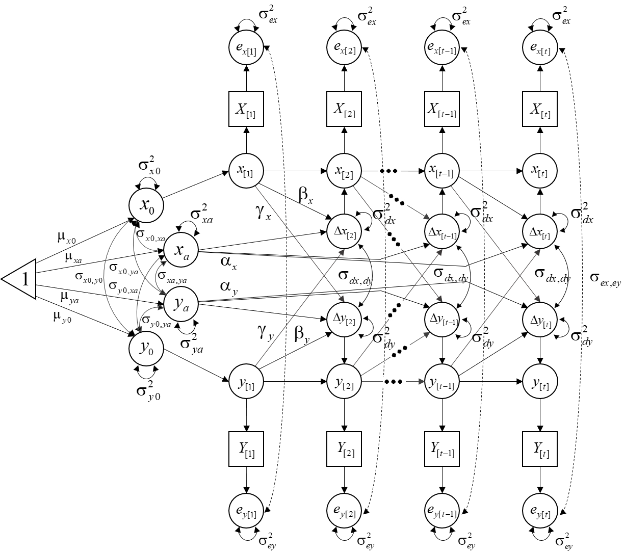
## Need help? See help(mxSummary)The Bivariate LCS model
Single indicator
Obtain the example database here: Download BLCSdata.txt
We will estimate the following model:
Step 1. Load the package and database:
library(OpenMx)
dfwide <- read.table("BLCSdata.txt")
Step 2. Define the variables of the model:
Tmax <- 5 # Number of measurement occasions
colnames(dfwide) <- c(paste0("X", 1:Tmax), paste0("Y",1:Tmax))

# Create the labels for the latent state at t=0, the additive component, the manifest scores, their corresponding latent scores, and the latent changes:
x0 <- "x0"
xa <- "xa"
y0 <- "y0"
ya <- "ya"
manif_X <- paste0("X", 1:Tmax)
manif_Y <- paste0("Y", 1:Tmax)
latent_x <- paste0("x", 1:Tmax)
latent_y <- paste0("y", 1:Tmax)
change_x <- paste0("Delta_x", 2:Tmax)
change_y <- paste0("Delta_y", 2:Tmax)
Step 3. Build the model:
BLCS.model <- mxModel("Bivariate LCS", type="RAM",
      manifestVars=c(manif_Y, manif_X),
      latentVars=c(x0, xa, y0, ya, latent_x, latent_y, change_x, change_y),
      mxData(observed = dfwide, type="raw"),

### LATENT STRUCTURE
      # 1 -> Initial factors and additive components (means)
      mxPath(from="one", to=c(x0, xa, y0, ya),
             arrows=1, free=TRUE, values= 0, labels=c("meanx0", "meanxa", "meany0", "meanya")),

      # (Co)variances of the initial factors and additive components
      mxPath(from="x0", arrows=2, free=TRUE, values=0, labels="varx0"),
      mxPath(from="xa", arrows=2, free=TRUE, values=0, labels="varxa"),
      mxPath(from="y0", arrows=2, free=TRUE, values=0, labels="vary0"),
      mxPath(from="ya", arrows=2, free=TRUE, values=0, labels="varya"),
      mxPath(from="x0", to="y0", arrows=2, free=TRUE, values=0, labels="covx0y0"),
      mxPath(from="x0", to="xa", arrows=2, free=TRUE, values=0, labels="covx0xa"),
      mxPath(from="x0", to="ya", arrows=2, free=TRUE, values=0, labels="covx0ya"),
      mxPath(from="xa", to="y0", arrows=2, free=TRUE, values=0, labels="covxay0"),
      mxPath(from="xa", to="ya", arrows=2, free=TRUE, values=0, labels="covxaya"),
      mxPath(from="y0", to="ya", arrows=2, free=TRUE, values=0, labels="covy0ya"),

      # Initial factor -> Initial latent score
      mxPath(from=x0, to=latent_x[1], arrows=1, free=FALSE, values=1),
      mxPath(from=y0, to=latent_y[1], arrows=1, free=FALSE, values=1),

      # Latent[t-1] -> Latent[t]
      mxPath(from=latent_x[1:(Tmax-1)], to=latent_x[2:Tmax], arrows=1, free=FALSE, values=1),
      mxPath(from=latent_y[1:(Tmax-1)], to=latent_y[2:Tmax], arrows=1, free=FALSE, values=1),

      # Additive component -> Change (alpha = 1)
      mxPath(from=xa, to=change_x, arrows=1, free=FALSE, values=1),
      mxPath(from=ya, to=change_y, arrows=1, free=FALSE, values=1),


      # Latent[t-1] -> Change[t] (self-feedbacks)
      mxPath(from=latent_x[1:(Tmax-1)], to=change_x, arrows=1, free=TRUE, values=0, labels="beta_x"),
      mxPath(from=latent_y[1:(Tmax-1)], to=change_y, arrows=1, free=TRUE, values=0, labels="beta_y"),

      # Latent[t-1] -> Change[t] (couplings)
      mxPath(from=latent_x[1:(Tmax-1)], to=change_y, arrows=1, free=TRUE, values=0, labels="gamma_y"),
      mxPath(from=latent_y[1:(Tmax-1)], to=change_x, arrows=1, free=TRUE, values=0, labels="gamma_x"),

      # Change -> Latent
      mxPath(from=change_x, to=latent_x[2:Tmax], arrows=1, free=FALSE, values=1),
      mxPath(from=change_y, to=latent_y[2:Tmax], arrows=1, free=FALSE, values=1),

### MEASUREMENT STRUCTURE
      # Latent -> Manifest
      mxPath(from=c(latent_x, latent_y), to=c(manif_X, manif_Y), arrows=1, free=FALSE, values=1),

      # Measurement errors variances and covariance
      mxPath(from=manif_X, arrows=2, free=TRUE, values=.5, labels="merX"),
      mxPath(from=manif_Y, arrows=2, free=TRUE, values=.5, labels="merY"),
      mxPath(from=manif_X, to=manif_X, arrows=2, free=TRUE, values=0, labels="covMer"))
Step 4. Estimate the model parameters:
BLCS.fit <- mxRun(BLCS.model)Click here to see the results
summary(BLCS.fit)## Summary of Bivariate LCS
##
## free parameters:
## name matrix row col Estimate Std.Error A
## 1 beta_x A Delta_x2 x1 0.37494095 0.012214135
## 2 gamma_y A Delta_y2 x1 -0.57279026 0.007822497
## 3 gamma_x A Delta_x2 y1 0.78274382 0.021090686
## 4 beta_y A Delta_y2 y1 -0.75220638 0.013225624
## 5 merY S Y1 Y1 0.28303669 0.005158571
## 6 covMer S X1 X1 0.37445849 0.007154220
## 7 varx0 S x0 x0 0.59738523 0.024795487
## 8 covx0xa S x0 xa -0.08172970 0.012532978
## 9 varxa S xa xa 0.25189317 0.013453275
## 10 covx0y0 S x0 y0 -0.09318767 0.014853277
## 11 covxay0 S xa y0 -0.08437976 0.010850833
## 12 vary0 S y0 y0 0.32163704 0.017177964
## 13 covx0ya S x0 ya 0.13963737 0.015606761
## 14 covxaya S xa ya 0.07196516 0.014304371
## 15 covy0ya S y0 ya 0.12871606 0.011974518
## 16 varya S ya ya 0.37146990 0.020059356
## 17 meanx0 M 1 x0 -1.04563007 0.021005908
## 18 meanxa M 1 xa -3.05760316 0.073351150
## 19 meany0 M 1 y0 3.36771530 0.017298754
## 20 meanya M 1 ya 2.48788716 0.047705826
##
## Model Statistics:
## | Parameters | Degrees of Freedom | Fit (-2lnL units)
## Model: 20 19780 50033.75
## Saturated: 65 19735 NA
## Independence: 20 19780 NA
## Number of observations/statistics: 1980/19800
##
## Information Criteria:
## | df Penalty | Parameters Penalty | Sample-Size Adjusted
## AIC: 10473.75 50073.75 50074.18
## BIC: -100113.30 50185.57 50122.03
## To get additional fit indices, see help(mxRefModels)
## timestamp: 2021-04-18 20:27:00
## Wall clock time: 0.433033 secs
## optimizer: SLSQP
## OpenMx version number: 2.19.1
## Need help? See help(mxSummary)Stochastic BLCS model
It is possible to extend the previous model to include innovation variances and covariance by just adding a new mxPath() to the already built BLCS.model:
stoch_BLCS.model <- mxModel(BLCS.model, # call the previous model
     # Dynamic error variances and covariance
     mxPath(from=change_x, arrows=2, free=TRUE, values=0, labels="derX"),
     mxPath(from=change_y, arrows=2, free=TRUE, values=0, labels="derY"),
     mxPath(from=change_x, to=change_y, arrows=2, free=TRUE, values=0, labels="covDer"))

# Run the new model:
stoch_BLCS.fit <- mxRun(stoch_BLCS.model)
Click here to see the results
summary(stoch_BLCS.fit)## Summary of Bivariate LCS
##
## free parameters:
## name matrix row col Estimate Std.Error A
## 1 beta_x A Delta_x2 x1 0.60288269 0.009715951
## 2 gamma_y A Delta_y2 x1 -0.24578344 0.006208989
## 3 gamma_x A Delta_x2 y1 0.95441632 0.018624155
## 4 beta_y A Delta_y2 y1 -0.39203653 0.012596048
## 5 merY S Y1 Y1 0.04548341 0.010143332
## 6 covMer S X1 X1 0.29555760 0.009483033
## 7 varx0 S x0 x0 0.61531651 0.024740008
## 8 covx0xa S x0 xa -0.18999044 0.015137135
## 9 varxa S xa xa 0.17806823 0.014258193
## 10 covx0y0 S x0 y0 -0.13762347 0.014417543
## 11 covxay0 S xa y0 -0.20543079 0.011616959
## 12 vary0 S y0 y0 0.45751709 0.018976062
## 13 covx0ya S x0 ya 0.03441336 0.006431347
## 14 covxaya S xa ya -0.11828754 0.005188054
## 15 covy0ya S y0 ya 0.03139110 0.005913824
## 16 varya S ya ya -0.06319358 0.006256364
## 17 derX S Delta_x2 Delta_x2 0.39226419 0.033374137
## 18 covDer S Delta_x2 Delta_y2 0.27089696 0.012865807
## 19 derY S Delta_y2 Delta_y2 0.48102413 0.021078158
## 20 meanx0 M 1 x0 -1.06660642 0.020642608
## 21 meanxa M 1 xa -3.32498894 0.072773121
## 22 meany0 M 1 y0 3.31622793 0.015933272
## 23 meanya M 1 ya 1.67278454 0.048363686
##
## Model Statistics:
## | Parameters | Degrees of Freedom | Fit (-2lnL units)
## Model: 23 19777 48893.06
## Saturated: 65 19735 NA
## Independence: 20 19780 NA
## Number of observations/statistics: 1980/19800
##
## Information Criteria:
## | df Penalty | Parameters Penalty | Sample-Size Adjusted
## AIC: 9339.064 48939.06 48939.63
## BIC: -101231.218 49067.65 48994.58
## To get additional fit indices, see help(mxRefModels)
## timestamp: 2021-04-18 20:27:01
## Wall clock time: 0.5549529 secs
## optimizer: SLSQP
## OpenMx version number: 2.19.1
## Need help? See help(mxSummary)Multiple Indicators
Obtain the example database here: Download MIBLCSdata.txt
We will estimate the following model: 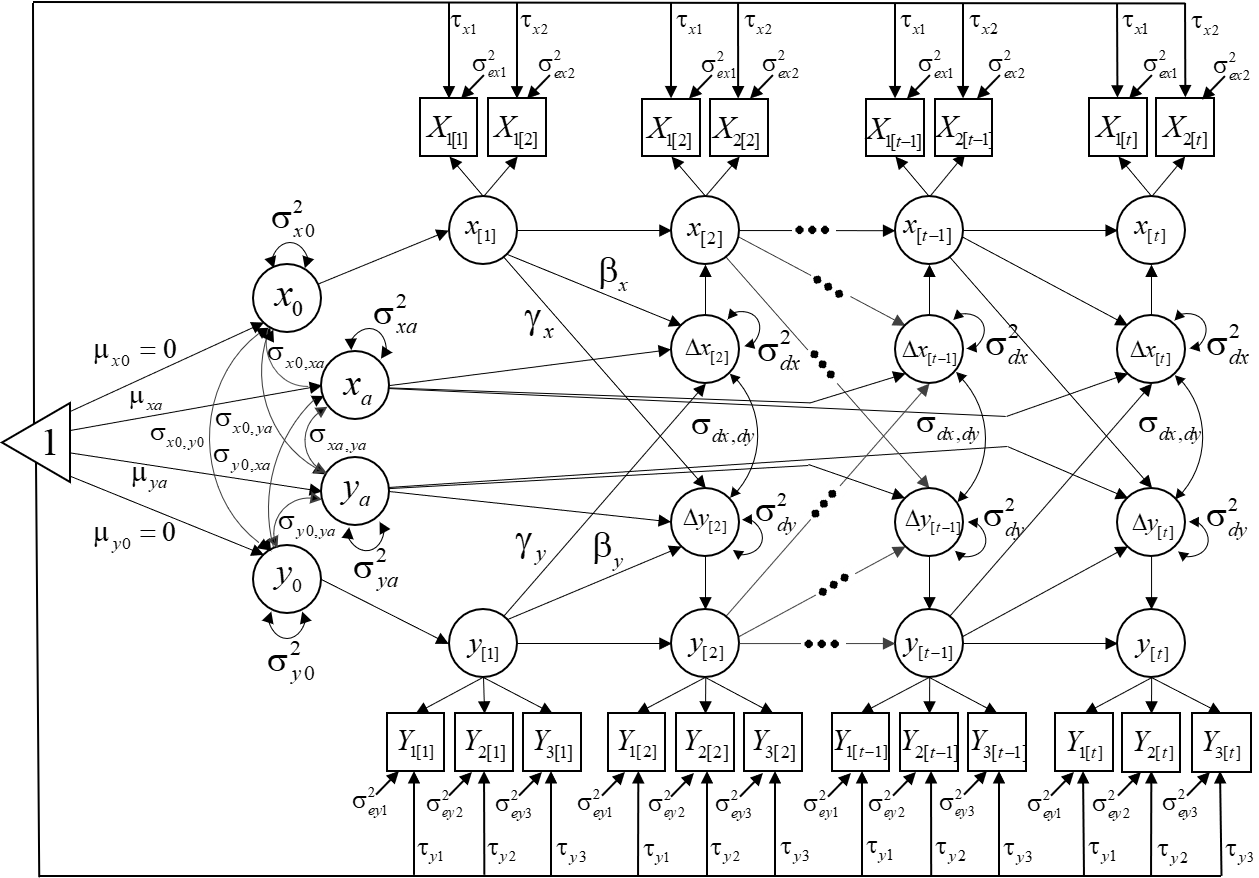
Step 1. Load the package and database:
library(OpenMx)
dfwide <- read.table("MIBLCSdata.txt")
Step 2. Define the variables of the model:
Tmax <- 5 # Number of measurement occasions
# Variables
x0 <- "x0"
xa <- "xa"
y0 <- "y0"
ya <- "ya"
indic_X1 <- paste0("X1_t", 1:Tmax)
indic_X2 <- paste0("X2_t", 1:Tmax)
indic_Y1 <- paste0("Y1_t", 1:Tmax)
indic_Y2 <- paste0("Y2_t", 1:Tmax)
indic_Y3 <- paste0("Y3_t", 1:Tmax)
latent_x <- paste0("x", 1:Tmax)
latent_y <- paste0("y", 1:Tmax)
change_x <- paste0("Delta_x", 2:Tmax)
change_y <- paste0("Delta_y", 2:Tmax)
Step 3. Build the model:
MI_BLCS.model <- mxModel("Bivariate LCS", type="RAM",
      manifestVars=c(indic_X1, indic_X2, indic_Y1, indic_Y2, indic_Y3),
      latentVars=c(x0, xa, y0, ya, latent_x, latent_y, change_x, change_y),
      mxData(observed = dfwide, type="raw"),

### LATENT STRUCTURE
      # 1 -> Initial factors and additive components (means)
      mxPath(from="one", to=c(xa, ya),
             arrows=1, free=TRUE, values= 0, labels=c("meanxa", "meanya")),

      # Covariance structure of the latent initial conditions

      mxPath(from="x0", arrows=2, free=TRUE, values=0, labels="varx0"),
      mxPath(from="xa", arrows=2, free=TRUE, values=0, labels="varxa"),
      mxPath(from="y0", arrows=2, free=TRUE, values=0, labels="vary0"),
      mxPath(from="ya", arrows=2, free=TRUE, values=0, labels="varya"),
      mxPath(from="x0", to="y0", arrows=2, free=TRUE, values=0, labels="covx0y0"),
      mxPath(from="x0", to="xa", arrows=2, free=TRUE, values=0, labels="covx0xa"),
      mxPath(from="x0", to="ya", arrows=2, free=TRUE, values=0, labels="covx0ya"),
      mxPath(from="xa", to="y0", arrows=2, free=TRUE, values=0, labels="covxay0"),
      mxPath(from="xa", to="ya", arrows=2, free=TRUE, values=0, labels="covxaya"),
      mxPath(from="y0", to="ya", arrows=2, free=TRUE, values=0, labels="covy0ya"),

      # Initial factor -> Initial latent score
      mxPath(from=x0, to=latent_x[1], arrows=1, free=FALSE, values=1),
      mxPath(from=y0, to=latent_y[1], arrows=1, free=FALSE, values=1),

      # Latent[t-1] -> Latent[t]
      mxPath(from=latent_x[1:(Tmax-1)], to=latent_x[2:Tmax], arrows=1, free=FALSE, values=1),
      mxPath(from=latent_y[1:(Tmax-1)], to=latent_y[2:Tmax], arrows=1, free=FALSE, values=1),

      # Additive component -> Change (alpha = 1)
      mxPath(from=xa, to=change_x, arrows=1, free=FALSE, values=1),
      mxPath(from=ya, to=change_y, arrows=1, free=FALSE, values=1),

      # Latent[t-1] -> Change[t] (self-feedbacks)
      mxPath(from=latent_x[1:(Tmax-1)], to=change_x, arrows=1, free=TRUE, values=0, labels="beta_x"),
      mxPath(from=latent_y[1:(Tmax-1)], to=change_y, arrows=1, free=TRUE, values=0, labels="beta_y"),

      # Latent[t-1] -> Change[t] (couplings)
      mxPath(from=latent_x[1:(Tmax-1)], to=change_y, arrows=1, free=TRUE, values=0, labels="gamma_y"),
      mxPath(from=latent_y[1:(Tmax-1)], to=change_x, arrows=1, free=TRUE, values=0, labels="gamma_x"),

      # Change -> Latent
      mxPath(from=change_x, to=latent_x[2:Tmax], arrows=1, free=FALSE, values=1),
      mxPath(from=change_y, to=latent_y[2:Tmax], arrows=1, free=FALSE, values=1),

      ## For the stochastic version, include:
      # Dynamic error variances and covariance (time-invariant)
      mxPath(from=change_x, arrows=2, free=TRUE, values=0, labels="derX"),
      mxPath(from=change_y, arrows=2, free=TRUE, values=0, labels="derY"),
      mxPath(from=change_x, to=change_y, arrows=2, free=TRUE, values=0, labels="covDer"),

## MEASUREMENT STRUCTURE
      # Factor loadings: Configural and weak invariance
      mxPath(from=latent_x, to=indic_X1, arrows=1, free=FALSE, values=1, labels="lambda_X1"),
      mxPath(from=latent_x, to=indic_X2, arrows=1, free=TRUE, values=0, labels="lambda_X2"),
      mxPath(from=latent_y, to=indic_Y1, arrows=1, free=FALSE, values=1, labels="lambda_Y1"),
      mxPath(from=latent_y, to=indic_Y2, arrows=1, free=TRUE, values=0, labels="lambda_Y2"),
      mxPath(from=latent_y, to=indic_Y3, arrows=1, free=TRUE, values=0, labels="lambda_Y3"),

      # Intercepts of the indicators: Strong invariance
      mxPath(from="one", to=indic_X1, arrows=1, free=TRUE, values=0, labels="tau_X1"),
      mxPath(from="one", to=indic_X2, arrows=1, free=TRUE, values=0, labels="tau_X2"),
      mxPath(from="one", to=indic_Y1, arrows=1, free=TRUE, values=0, labels="tau_Y1"),
      mxPath(from="one", to=indic_Y2, arrows=1, free=TRUE, values=0, labels="tau_Y2"),
      mxPath(from="one", to=indic_Y3, arrows=1, free=TRUE, values=0, labels="tau_Y3"),

      # Measurement error variances (time-invariant)
      mxPath(from=indic_X1, arrows=2, free=TRUE, values=0, labels="mer_X1"),
      mxPath(from=indic_X2, arrows=2, free=TRUE, values=0, labels="mer_X2"),
      mxPath(from=indic_Y1, arrows=2, free=TRUE, values=0, labels="mer_Y1"),
      mxPath(from=indic_Y2, arrows=2, free=TRUE, values=0, labels="mer_Y2"),
      mxPath(from=indic_Y3, arrows=2, free=TRUE, values=0, labels="mer_Y3")
            )
Step 4. Estimate the model parameters:
MI_BLCS.fit <- mxRun(MI_BLCS.model)Click here to see the results
summary(MI_BLCS.fit)## Summary of Bivariate LCS
##
## free parameters:
## name matrix row col Estimate Std.Error A
## 1 lambda_X2 A X2_t1 x1 0.90046698 0.001748088
## 2 beta_x A Delta_x2 x1 0.35445677 0.008555211
## 3 gamma_y A Delta_y2 x1 -0.54843332 0.006541111
## 4 lambda_Y2 A Y2_t1 y1 0.85028627 0.001980699
## 5 lambda_Y3 A Y3_t1 y1 0.74700598 0.002464167
## 6 gamma_x A Delta_x2 y1 0.64372718 0.008413555
## 7 beta_y A Delta_y2 y1 -0.74664977 0.006348337
## 8 mer_X1 S X1_t1 X1_t1 0.19596694 0.004017893
## 9 mer_X2 S X2_t1 X2_t1 0.14597864 0.003124073
## 10 mer_Y1 S Y1_t1 Y1_t1 0.24607402 0.004516764
## 11 mer_Y2 S Y2_t1 Y2_t1 0.09962459 0.002372177
## 12 mer_Y3 S Y3_t1 Y3_t1 0.29526091 0.004673245
## 13 varx0 S x0 x0 0.60023545 0.021157471
## 14 covx0xa S x0 xa -0.12542800 0.011056446
## 15 varxa S xa xa 0.23584393 0.011767043
## 16 covx0y0 S x0 y0 -0.10151284 0.012587120
## 17 covxay0 S xa y0 -0.09604707 0.008997802
## 18 vary0 S y0 y0 0.38401310 0.014522304
## 19 covx0ya S x0 ya 0.15296666 0.012578506
## 20 covxaya S xa ya 0.09407315 0.011474081
## 21 covy0ya S y0 ya 0.13885946 0.010102650
## 22 varya S ya ya 0.33345988 0.016930950
## 23 derX S Delta_x2 Delta_x2 0.20042123 0.009299487
## 24 covDer S Delta_x2 Delta_y2 0.02598560 0.004831832
## 25 derY S Delta_y2 Delta_y2 0.14808508 0.005028817
## 26 tau_X1 M 1 X1_t1 -0.55146672 0.019248658
## 27 tau_X2 M 1 X2_t1 -0.48769254 0.017242585
## 28 tau_Y1 M 1 Y1_t1 1.28709245 0.016988246
## 29 tau_Y2 M 1 Y2_t1 1.10167744 0.013509374
## 30 tau_Y3 M 1 Y3_t1 0.98877077 0.014625937
## 31 meanxa M 1 xa -2.55366868 0.015082660
## 32 meanya M 1 ya 2.55835593 0.016196764
##
## Model Statistics:
## | Parameters | Degrees of Freedom | Fit (-2lnL units)
## Model: 32 49468 90302.35
## Saturated: 350 49150 NA
## Independence: 50 49450 NA
## Number of observations/statistics: 1980/49500
##
## Information Criteria:
## | df Penalty | Parameters Penalty | Sample-Size Adjusted
## AIC: -8633.652 90366.35 90367.43
## BIC: -285201.925 90545.26 90443.59
## To get additional fit indices, see help(mxRefModels)
## timestamp: 2021-04-18 20:27:04
## Wall clock time: 2.345692 secs
## optimizer: SLSQP
## OpenMx version number: 2.19.1
## Need help? See help(mxSummary)